Day 2:  Quicksort The Ultimate Guide to the Divide and Conquer Champion

Quicksort is the “Gold Standard” of sorting algorithms. Efficient, in-place, and remarkably fast, it is the backbone of many standard libraries (like C++ std::sort). This guide breaks down the complex logic of quicksort into a streamlined, high-performance reference for developers.

1. What is Quicksort? (The High-Level View)

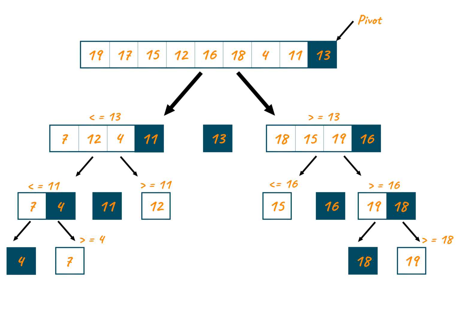
Quicksort is a Divide and Conquer algorithm. It works by selecting a “pivot” element from the array and partitioning the other elements into two sub-arrays, according to whether they are less than or greater than the pivot.

The Three-Step Process:

1. Pivot Selection: Pick an element to act as the “benchmark.”
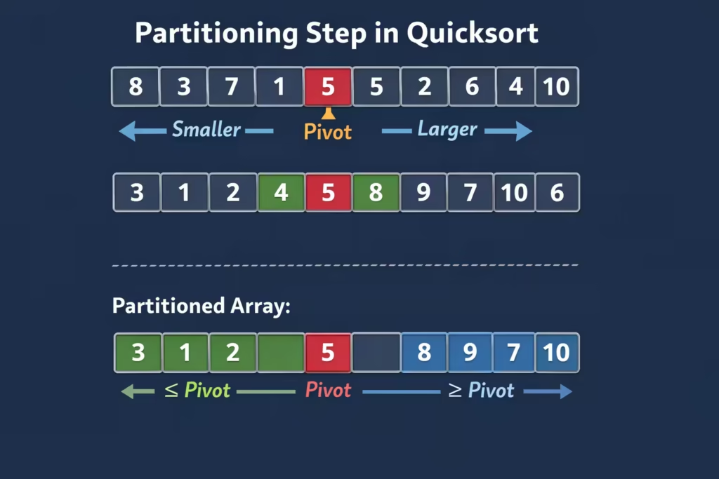
2. Partitioning: Move all smaller elements to the left of the pivot and larger ones to the right.
3. Recursion: Apply the same logic to the left and right sides until the base case (size 0 or 1) is reached.

2. Pivot Selection: Strategies for Speed

The efficiency of Quicksort depends almost entirely on how you pick your pivot. If you pick a pivot that splits the array exactly in half, the algorithm flies. If you pick the smallest or largest element every time, it crawls.

• Fixed Pivot: Always picking the first or last element. (Risky! Leads to $O(n^2)$ on already sorted data).
• Random Pivot: Choosing an index at random. This is the industry standard to avoid worst-case scenarios.
• Median-of-Three: Taking the median of the first, middle, and last elements to ensure a more balanced split.

3. Deep Dive into Partitioning Schemes

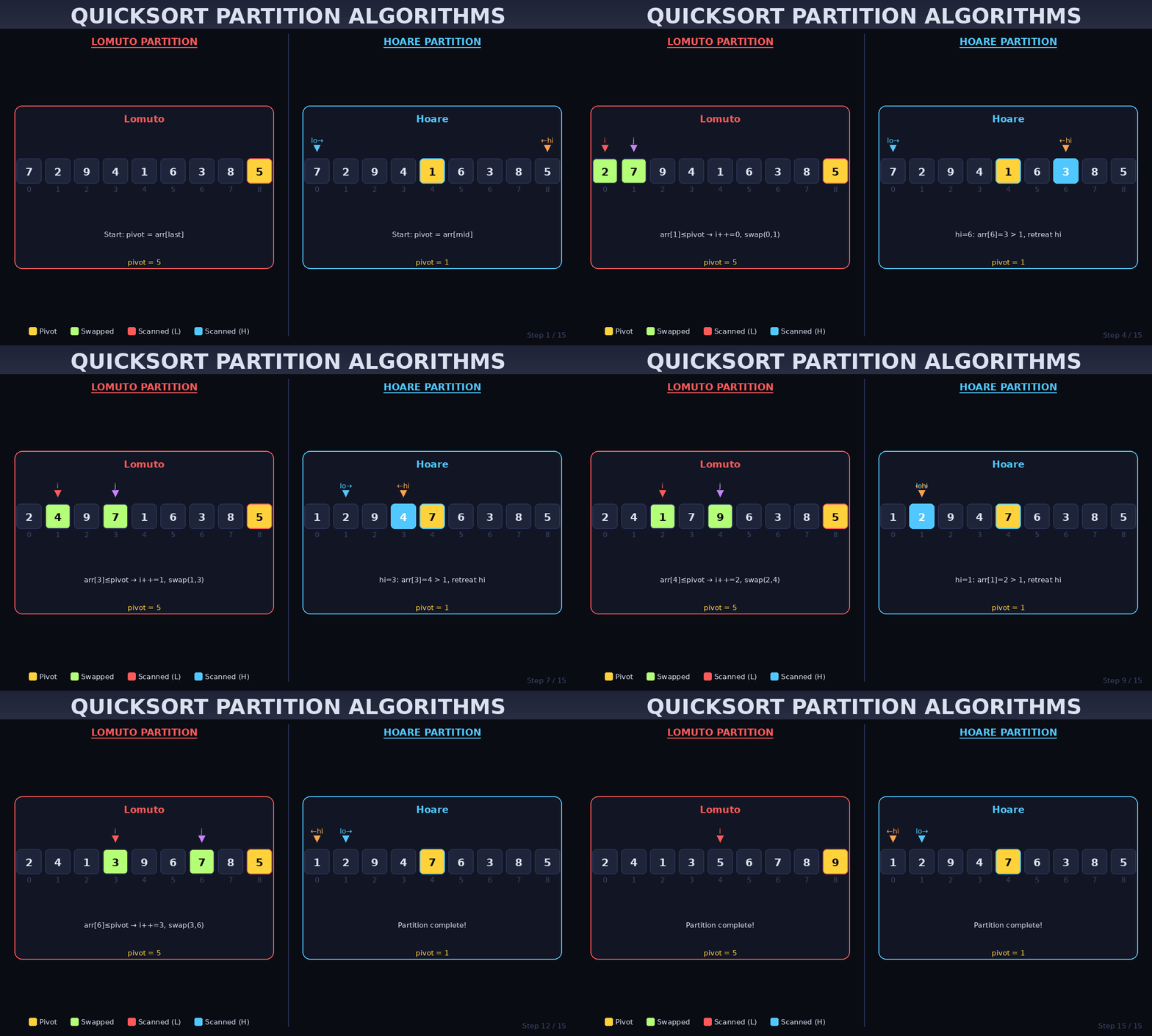
Partitioning is where the actual “sorting” happens. While there are several methods, these two are the most famous:

Lomuto Partition (Simple)

This method is the easiest to implement. It uses a single pointer that moves across the array, swapping elements that are smaller than the pivot.

• Best for: Beginners and educational purposes.

Hoare Partition (Performance)

The Hoare scheme uses two pointers starting from the ends and moving toward each other. It performs fewer swaps on average than Lomuto.

• Best for: Production-grade libraries and high-speed applications.

4. Performance and Complexity Analysis

Understanding Quicksort’s performance is critical for technical interviews and system design.

Scenario	Time Complexity	Auxiliary Space
Best Case	$O(n \log n)$	$O(\log n)$
Average Case	$O(n \log n)$	$O(\log n)$
Worst Case	$O(n^2)$	$O(n)$

Why is Quicksort “Cache-Friendly”?

Unlike Merge Sort, which requires extra arrays to store data, Quicksort is in-place. It works directly on the original memory block, making it much faster in practice due to how CPU caches function.

5. Python Implementation

The “Pythonic” Way (Easy to Read)

This version uses list comprehensions. It is highly readable because it mirrors the “Divide and Conquer” logic exactly. However, note that this version uses extra memory to create new lists.

def quicksort(arr):
    # Base case: arrays with 0 or 1 element are already "sorted"
    if len(arr) <= 1:
        return arr
    
    # Selecting the middle element as the pivot
    pivot = arr[len(arr) // 2]
    
    # Partitioning
    left = [x for x in arr if x < pivot]
    middle = [x for x in arr if x == pivot]
    right = [x for x in arr if x > pivot]
    
    # Recursive calls
    return quicksort(left) + middle + quicksort(right)

# Test the function
data = [10, 7, 8, 9, 1, 5]
sorted_data = quicksort(data)
print(f"Sorted Array: {sorted_data}")

The Efficient Way (In-Place / Lomuto)

This version sorts the array in-place, meaning it doesn’t create new lists. This is much better for large datasets because it saves memory ($O(1)$ auxiliary space excluding the recursion stack).

def partition(arr, low, high):
    # We choose the last element as the pivot
    pivot = arr[high]
    i = low - 1  # Pointer for the greater element

    for j in range(low, high):
        # If current element is smaller than the pivot
        if arr[j] <= pivot:
            i += 1
            # Swap elements
            arr[i], arr[j] = arr[j], arr[i]

    # Swap the pivot element with the greater element specified by i
    arr[i + 1], arr[high] = arr[high], arr[i + 1]
    
    # Return the position where partition is done
    return i + 1

def quick_sort(arr, low, high):
    if low < high:
        # Find pivot element such that
        # element smaller than pivot are on the left
        # element greater than pivot are on the right
        pi = partition(arr, low, high)

        # Recursive call on the left of pivot
        quick_sort(arr, low, pi - 1)

        # Recursive call on the right of pivot
        quick_sort(arr, pi + 1, high)

# Test the function
data = [10, 7, 8, 9, 1, 5]
quick_sort(data, 0, len(data) - 1)
print(f"In-place Sorted Array: {data}")

Which one should you use?

Feature	Pythonic Version	In-Place (Lomuto)
Readability	⭐⭐⭐⭐⭐ (Very easy)	⭐⭐⭐ (Requires pointer logic)
Memory	❌ High ($O(n)$ extra space)	✅ Low ($O(\log n)$ space)
Speed	Fast for small lists	Faster for large datasets
Stability	Can be made stable	Usually unstable

6. Real-World Applications

Quicksort isn’t just a classroom exercise. You’ll find it in:

• Commercial Databases: For fast record indexing.
• Graphics Engines: Sorting objects by depth for rendering.
• Standard Libraries: Used in C’s qsort and parts of C++’s std::sort.

7. Summary: Pros vs. Cons

• Pros: Extremely fast average case, uses very little extra memory, easy to parallelize.
• Cons: Not “stable” (equal elements might swap order), $O(n^2)$ worst-case risk if not implemented carefully.

Reference & Further Reading

• GeeksforGeeks: Quick Sort Algorithm Guide
• Introduction to Algorithms (CLRS)
• Sorting Visualizer: Quicksort in Motion